It’s finally time for Part 4! Now that we know how to design and numerically solve simple ODE models it’s time to take a look at how to fit these models to empirical data. It is important to remember that we design models to simulate real behavior. Thus, it is important to be able to tie our ODE equations to the real system we are trying to model. We do this by choosing values for our model parameters that makes the system behave similar to real world behavior. This lesson continues in Part 4B.

Before we get started, I encourage you to take a look at the previous lessons to get caught up. Lesson 1 discussed the meaning of an Ordinary Differential Equation and looked at some simple methods for solving these equations. Lesson 2 looked at the Runge-Kutta approach to solving ODEs and showed us how to use Matlab’s built in function to do so. Lesson 3 looked at two sample multi-population ODE models and explored how to interpret ODE models of living systems. The next planned post in this series, Lesson 5, will look at complex chaotic systems and play with the concept of strange attractors.

Today, we’re going to look at a made up infection that spreads through a very isolated town of 50,000 people. Because the infection was not severe, the local health board estimated that one out of every 100 people who were infected came in for a visit. The health board then went to the local clinics and hospitals to see how many people got a check-up each day. It was later discovered the disease was introduced to the town by a woman returning from a business trip. She returned and entered the town on what we will call ‘Day 0’. Here are the reported health visits by day:

Day	Visits
2	1
4	5
5	35
6	150
7	250
8	260
10	160
12	90
14	45

Now let’s suppose we are medical researchers who want to figure out how long it takes for an infected individual to recover from this infection. Guess what? We already have everything we need to know!

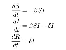
We will use our SIR model from the previous lesson to model this infection. This model is very simple and can be expended, but we will not worry about that in this lesson. The SIR equations are as follows:

Again, S represents the susceptible population, I represents the infected population, and R represents the recovered population. Note that in this instance, we have empirical data relating to the infected population versus time.

We will code this equation up similar to the way we did it in the previous lesson. The difference here is that we will use global declarations to allow us to pass in parameter values from outside our SIR function.

% sir.m 
%
% Implements an SIR infection model
% dS/dt = -beta SI
% dI/dt = beta SI - delta I
% dR/dt = delta I
%
% Inputs:
% t - Time variable: not used here because our equation 
%     is independent of time, or 'autonomous'.
% x - Independent variable: this contains three
%     populations (S, I, and R)
% Output:
% dx - First derivative: the rate of change of the populations
function dx = sir(t, x) 
  global beta delta; 

  dx = [0; 0; 0]; 

  dx(1) = -beta * x(1) * x(2); 
  dx(2) = beta * x(1) * x(2) - delta * x(2); 
  dx(3) = delta * x(2);

Now, the trick is to choose values for β and δ that makes our model behave similarly to the data. More specifically, we want to find β and δ that minimize the squared error between the simulated infected population and the data. We choose to minimize the squared error to make the fitting algorithm balance the error of every point (instead of ignoring a point or two to the benefit of the others). Finding these two values is what’s known as non-linear function optimization. In this case our function is the squared error between the model and the data and the optimization we are trying to perform is the minimization of the error.

Unfortunately, there is no magic solution for this technique. Because the function is non-linear, we cannot simply solve for β and δ. Fortunately, there are techniques that make this search easier. I will discuss two in this lesson: the Levenberg-Marquardt algorithm and the Genetic Algorithm (GA).

The Levenberg-Marquardt algorithm is a gradient-descent method and thus can get stuck in local-minima. It also requires the user to specify an initial guess. Thus, when dealing with very volatile equations a GA may be a better choice.

Matlab has a built-in implementation of the Levenberg-Marquardt algorithm called nlinfit. To use it we must know the data we’re trying to fit to, the function we’re trying to fit, and an initial guess for our parameters. Let’s go through these one step at a time.

The data we are trying to fit to is contained in the table above. We simply need to enter that data into Matlab:

day = [2 4 5 6 7 8 10 12 14]; 
sick = [1 5 35 150 250 260 160 90 45];

Next, we need to define a function that represents our equation. The equation takes in an array with the free parameters (β and δ) and a list of time points to find values for. It should return an array of values that correspond to the time points given. We will create this function by combining ode15s and interp1. ode15s works similarly to ode45 but behaves better when evaluating ‘stiff’ functions (functions that have very steep gradients). Depending on our values for β and δ, ode45 may struggle, so for this lesson we will be sticking with ode15s.

% infection.m 
%
% Returns expected infection values given a set of time points and 
%   coefficients 
% Inputs: 
% a – List of free parameter values 
% x – List of time points of interest 
% Output: 
% y – A list of expected number of infected people for each time 
%     point in ‘x’. 
function y = infection(a, x) 
  % Define beta and delta as globals so we can pass the values into the 
  % ‘sir’ function. 
  global beta delta; 
  beta = a(1); 
  delta = a(2); 

  % Solve our model. The initial population was 50,000 healthy 
  % individuals and one infected person. Run the model until the 
  % last time point we are concerned about. 
  % (we are assuming x is ordered). 
  [t, y] = ode15s(‘sir’, [0 x(end)], [50000, 1, 0]); 

  % Recall that we are interested only in the infected population. 
  % We will use the built-in interpolation function interp1 to get 
  % values of infected people at that correspond to the proper time 
  % points. 
  y = interp1(t, y(:,2), x);

Before we start, we also want to set the display mode so that we can watch the algorithm proceed. To do so we use the statset function.

options = statset('Display', 'iter');

Remember that our ‘sick’ array counts only people who sought help. We want to multiply it by 100 to get an estimate of how many people were actually sick at that time. Finally, we also need to provide a starting guess for the two parameters. Let’s try 0.0005 for β and 0.1 for δ. Now it’s just a simple matter of passing in all the correct arguments to nlinfit.

[values] = nlinfit(day, sick*100, ‘infection’, [.00005 .1], options)

After several iterations, we get a result:

values = 0.0000 0.3290 

A value of zero for β? Wait one sec. Matlab’s default behavior is to only show four decimal places for each number. We can fix that by changing the display format:

format long

Now take a new look at the values:

values = 0.000040293800490 0.329045768752125

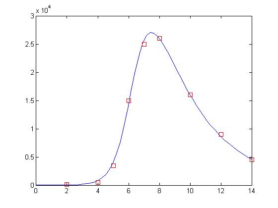
That’s more like it! The answer was there all along. Since values holds our parameters, this means that we have a value of approximately 0.00004 for β and approximately 0.329 for δ. Let’s take a look at how well these values perform:

% Declare as global so the values can be passed into the SIR function 
global beta delta; 

% Set beta and delta to the values found by nlinfit 
beta = values(1); 
delta = values(2); 

% Evaluate the ODE with the new values for beta and delta 
[t, y] = ode15s(‘sir’, [0 14], [50000 1 0]); 

% Display the results 
plot(t, y(:,2), ‘-b’, day, sick*100, ‘rs’)

And what a fit it is! It’s almost as though the data points were deliberately manufactured for this lesson!

With such a good fit, we should use nlinfit all the time, yes? Well, did anyone else notice that our initial guess was suspiciously close to the answer? Who guesses .00005 for β off the top of their head? What happens if we have no clue what β and δ should be? What happens if our initial guess is just 1 for each of them?

[values] = nlinfit(day, sick*100, ‘infection’, [1 1], options)

gives us these values:

values = 1.004882437649172 1.000088843687306

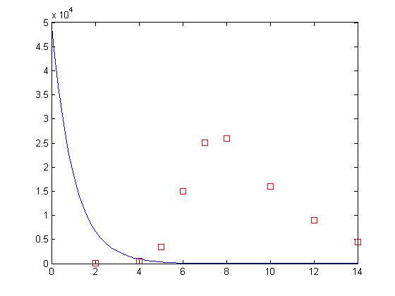
That’s suspiciously close to where we started! But, maybe it’s still right. Let’s take a look:

beta = values(1); 
delta = values(2); 

[t, y] = ode15s(‘sir’, [0 14], [50000 1 0]); 

plot(t, y(:,2), ‘-b’, day, sick*100, ‘rs’)

Whoops! What happened? The Levenberg-Marquardt algorithm implemented by nlinfit is a type of gradient descent algorithm. It works by looking at the error of the fit to the error of fits using slightly different values for the parameters. In doing so, it gets a small picture of the fitness landscape surrounding its current position. From there, the algorithm determines which direction results in the highest improvement in the error and then takes a step in that direction and repeats. This process works very well if there is a nice smooth slope leading to the best solution. Unfortunately, when dealing with non-linear systems this is not usually the case.

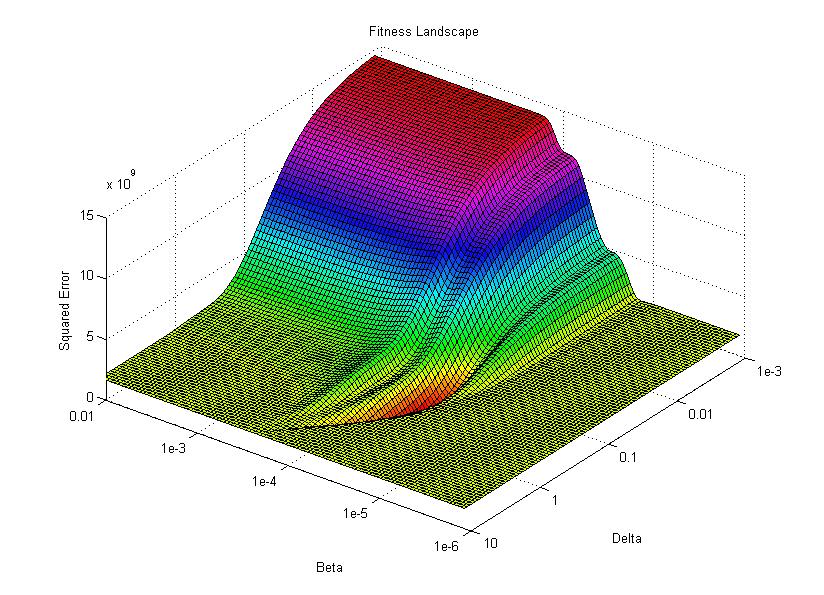
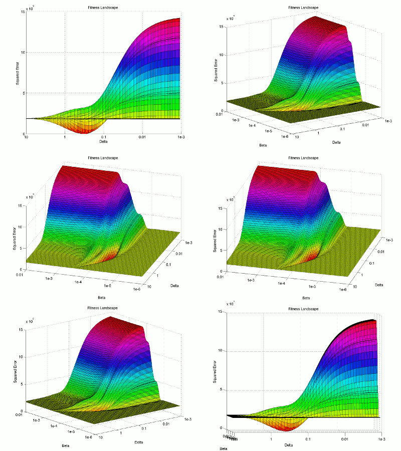
Let’s take a look at the fitness landscape around the solution. I will use logarithmic plotting so we can represent many orders of magnitude in a single graph. I’m not going to explain my steps in quite as much detail here as I mostly just want to look at the resulting figure.

% Generate a 3D Mesh, one point at a time 
for i=[1:101] 
  for j=[1:101] 
    % Transform beta and delta into log-space 
    b = 10^(.04*j-6); 
    d = 10^(.04*i-3); 
    
    % Get the estimates for the given beta and delta 
    points = infection([b d], day); 

    % Calculate the error as the sum of the squared residuals 
    error(i,j) = sum((100*sick – points).^2); 
  end 

  % Display a countdown as this is a long process. 
  disp(101-i); 
end

I then use the surface plotting command to generate the 3D image of the fitness landscape. I used the rotation tool to adjust the viewing angle (which you can also do with the view command) and adjusted the color map to better highlight the global minimum (the red trough).

For this image, the two base dimensions represent possible values for β and δ. The height of the surface at any point measures the error between the model and the data for those two values of β and δ. Thus, our first values, 0.00004 and 0.33 correspond to a low point on the graph (which is what we want). Conversely, the values 1.0 and 1.0 have a worse error and thus correspond to a higher point on the graph. In this case, β = 1.0 isn’t represented on the graph, but the point (1.0, 1.0) will lie on the flat yellow surface. The flat yellow surface corresponds to the cases where the model effectively predicts zero infections over the two week span.

Hopefully this figure will help illustrate why there was such a difference in our results given our two different starting points. Because nlinfit is a gradient descent algorithm, it acts similarly to a ball rolling down a hill. If our goal is to drop a ball on the above surface and have it roll into the red basin, we have to be very selective of where we drop it. Because our first guess of 0.00005 and 0.1 was within the main basin of attraction, nlinfit was able to find the global minimum. Unfortunately, the range of values that will lead to the proper solution is tiny compared to the search space. This will always be a problem for gradient descent algorithms operating on a non-linear function. Thus, we will turn to genetic algorithms as an alternative search method that performs a bit better on bumpy landscapes. But, since this post is already way too long, I am going to split this lesson into two parts, so please stay tuned for Lesson 4B, where I will discuss how to implement a genetic algorithm!

Until then, here’s a bonus snippet of code I used to generate individual frames for the following animation.

% Display the fitness landscape surface(error); 
for i=[0:30] 
  ang = 180 + 3*i;   % Rotate horizontally 
  elv = 45 – 1.5*i;  % Rotate vertically 
  view(ang, elv);    % Set the viewing angle 

  % Create a new file name for the new frame 
  name = sprintf(‘frames/frame-%02d.png’, i); 

  % Save the current figure as a png file using the 
  % file name specified above. 
  print(‘-dpng’, name); 
end

Thank you. This lesson continues in Part 4B as we look at other ways to do non-linear function optimization!