And so we reach the end. We will wrap up this series with a look at the fascinating Lorenz Attractor. Like the logistic map of the previous lesson, the Lorenz Attractor has the structure and behavior of a complex system. Unlike the logistic map, the Lorenz Attractor is defined by a system of first order autonomous ordinary differential equations. Thus, it is a perfect example to use for this last lesson where we examine the importance of error tolerance in evaluation chaotic systems of ODEs.

This is the second part of a two part lesson of a five part series. The first part of this lesson begins here. If you have not read the previous lessons in the series, I encourage you to start there (at least read through Part 2). Lesson 1 discussed the meaning of an Ordinary Differential Equation and looked at some simple methods for solving these equations. Lesson 2 looked at the Runge-Kutta approach to solving ODEs and showed us how to use Matlab’s built in function to do so. Lesson 3 looked at two sample multi-population ODE models and explored how to interpret ODE models of living systems. Lesson 4 examined non-linear optimization approaches to fitting ODE modeled systems to empirical data.

To begin, we need to define our ODEs. The Lorenz System is made up of the following three interrelated differential equations:

The equations are made up of three populations: x, y, and z, and three fixed coefficients: sigma, rho, and beta. Remembering what we discussed previously, this system of equations has properties common to most other complex systems. First, it is non-linear in two places: the second equation has a xz term and the third equation has a xy term. It is made up of a very few simple components. Although difficult to see until we plot the solution, the equation displays broken symmetry on multiple scales. Because the equation is autonomous (no t term in the right side of the equations), there is no feedback in this case.

This system’s behavior depends on the three constant values chosen for the coefficients. It has been shown that the Lorenz System exhibits complex behavior when the coefficients have the following specific values: sigma = 10, rho = 28 ,and beta = 8/3. We now have everything we need to code up the ODE into Matlab:

% lorenz.m
%
% Imlements the Lorenz System ODE
%   dx/dt = sigma*(y-x)
%   dy/dt = x*(rho-z)-y
%   dz/dt = xy-beta*z
%
% Inputs:
%   t - Time variable: not used here because our equation
%       is independent of time, or 'autonomous'.
%   x - Independent variable: has 3 dimensions
% Output:
%   dx - First derivative: the rate of change of the three dimension
%        values over time, given the values of each dimension
function dx = lorenz(t, x)

% Standard constants for the Lorenz Attractor
sigma = 10;
rho = 28;
beta = 8/3;

% I like to initialize my arrays
dx = [0; 0; 0];

% The lorenz strange attractor
dx(1) = sigma*(x(2)-x(1));
dx(2) = x(1)*(rho-x(3))-x(2);
dx(3) = x(1)*x(2)-beta*x(3);

We can now quickly generate a solution. I have picked a starting point of [10 10 10] and I encourage you to play around with other starting points. Because this is a system of three equations, the solution can be plotted in three dimensions. Because the shape of the solution is somewhat complex, I created a script to generate a rotating animation of the shape. The following lines of code generate 60 separate png files (one for each frame).

% Generate Solution
[t, y] = ode45('lorenz', [0 20], [10 10 10]);

% Create 3d Plot
plot3(y(:,1), y(:,2), y(:,3));

for i=1:60
      
    view(6*i, 40);   % Rotate the view

    set(gca, 'XLim', [-20 20])
    set(gca, 'YLim', [-25 25])
    set(gca, 'ZLim', [0 50])

    % Remove the axes
    axis off
    
    % Generate the file name for the new frame
    name = sprintf('frames/frame-%02d.png', i); 
    
    % Save the current figure as a png file using the 
    % file name specified above. 
    print('-dpng', name); 
end

I then use the Linux ImageMagick converter to combine the frames into a looping animated gif. This is a Linux command line command, not a Matlab command.

convert -delay 5 -loop 0 -resize 25% -depth 4 frame*.png lorenz.gif

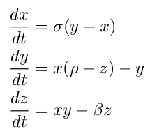
Here is the result!

Pretty cool, huh? The weird horizontal ‘bouncing’ seen in the animation is an artifact of how Matlab scales up its figures to fit the size of the window frame.

Anyway, let’s take a look. This image actually shows very similar behavior to last lesson’s logistic map solution. Without testing, I will assure you that the behavior is similarly sensitive to initial conditions (although we will not explore this feature here). There is some interesting emergent behavior as we see an almost orderly orbit around two main basins of attraction. Finally we see that the system does seem to be bounded within a specific region of space. What makes this system a strange attractor (just like the logistic map) is that even though the system is bounded, the orbit never exactly repeats itself.

The last lesson focused on how complex systems are sensitive to initial conditions. It turns out that complex systems are just sensitive in general. This time we will look at how this system is sensitive to the relative error tolerance of the ODE solver itself, in this case ode45. If you haven’t yet, you should take the time to review Lesson 2 where I discuss variable step sized ODE solver algorithms and look at how to set the tolerances of Matlab’s ODE solver.

To quickly review, ODE solvers take a step by step approach to generating a numerical solution to the ODE in question. To do so, a solution is generated by a fourth-order approximation for a given step size. Then, an approximate measure of the error of this solution is generated by using a more accurate fifth-order solution. If the error is too large, the step size is shortened and the algorithm makes a new approach at a solution (just one that is closer to where it started this time). This repeats until a solution is generated that is within the desired error tolerance.

It turns out that Matlab allows you to choose how forgiving you want your solver to be. You can set the relative error tolerance (‘RelTol’) and the absolute error tolerance (‘AbsTol’). For this example I will simply change the relative error tolerance. The default relative error tolerance is 0.001. I will lower that tolerance down to 1e-6 and compare the two solutions. In the following examples, the blue solution is generated using the 1e-6 relative tolerance. We set the error tolerance using the odeset function. Then we evaluate the solutions while passing in the returned value from the odeset function. Make note that in this example, the two solutions are using the exact same set of equations and starting at the exact same point.

>> options = odeset('RelTol', 1e-6);
>> [t,y] = ode45('lorenz', [0 50], [10 10 10], options);
>> options = odeset('RelTol', 1e-3);
>> [t2,y2] = ode45('lorenz', [0 50], [10 10 10], options);
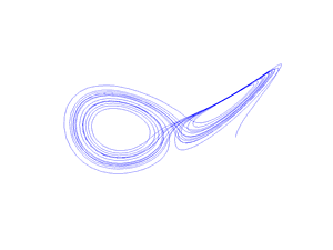
>> figure('Position',[100 100 800 600])
>> plot3(y(:,1),y(:,2),y(:,3), 'b', y2(:,1),y2(:,2),y2(:,3),'r')
>> view(45, 40)

Here is our result:

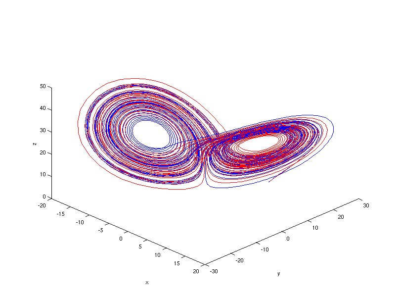
As you can see, the two solutions do seem to diverge. You can see it somewhat clearly in the inner part of the orbits, where one shows mostly blue and the other red. Still, it’s tricky to see exactly how quickly and where the two diverge. To get a better look at it, we will split the 3D graph into three separate graphs, one for each dimension.

>> figure('Position',[100 100 900 900])
>> subplot(3, 1, 1)
>> plot(t, y(:,1), 'b', t2, y2(:,1), 'r')
>> xlabel('t')
>> ylabel('x')
>> subplot(3, 1, 2)
>> plot(t, y(:,2), 'b', t2, y2(:,2), 'r')
>> xlabel('t')
>> ylabel('y')
>> subplot(3, 1, 3)
>> plot(t, y(:,3), 'b', t2, y2(:,3), 'r')
>> xlabel('t')
>> ylabel('z')

and again, here is our result:

Keep in mind that this is the exact same graph as the previous figure, just plotted differently. Here we can indeed see that the two solutions diverge very rapidly (although rapidly may be a misnomer as we are ignoring units in this lesson). Blue and red seem to diverge somewhere between time 5 and 10, and while they do come back into close proximity, they never join back together (just like our logistic map example).

How did this difference happen? Recall what I said about how a higher error tolerance forces the numerical solver to take smaller steps. In each case, the solver went from time 0 to time 50. But, let’s see how many steps each took to get there. We can simply look at the length of the output array of each:

>> length(t)

ans =

       10577

>> length(t2)

ans =

        2969

Thus, the same solver, solving the same equation, starting at the same starting point, took over 3.5 times as many steps than the default approach when using a higher error tolerance. Furthermore, not only did it take more steps and presumably generate a more accurate solution, after a short period of similarity, the more accurate solver generated a completely different solution than the default solver! The interesting question is to ask, how quickly did our `good’ solver diverge from the real solution? If there’s any lesson to take away from Part 5 of this series, it should be to always question the results of your numerical solutions to ODEs that describe complex and/or chaotic systems. It only takes small missteps for your solution to rapidly diverge from the actual solution.

That wraps up our series on ordinary differential equations in Matlab. Thanks for reading!