Welcome to Modeling with ODEs in Matlab – Part 4B! The previous post, Part 4A, introduced the idea of fitting ODE coefficients to empirical data. We saw that proper use of the nlinfit function combined with ode45 or ode15s allows us to fit a model to data when given a good initial estimate of the parameter values. Unfortunately, this approach does not work as well if the initial guess is not within the basin of attraction of the best fit. Today we will look at a new approach to function optimization: Genetic Algorithms (GAs). Genetic Algorithms are part of a search family I like to call “intelligent randomized search”, which also includes techniques such as Simulated Annealing and Particle Swarm Optimization.

If you have not read the previous posts in this series, I encourage you to look at them first. Lesson 1 discussed the meaning of an Ordinary Differential Equation and looked at some simple methods for solving these equations. Lesson 2 looked at the Runge-Kutta approach to solving ODEs and showed us how to use Matlab’s built in function to do so. Lesson 3 looked at two sample multi-population ODE models and explored how to interpret ODE models of living systems. The next planned post in this series, Lesson 5, will look at complex chaotic systems and play with the concept of strange attractors.

Continuing from last time, we want to develop a technique that allows us to get ODE parameter values from empirical data. More specifically, we want to find parameter values that when applied to our ODE model generate behavior that mimics the observed data. Contrary to Lesson 4A, we want a technique that is robust enough to traverse a complex non-linear search space without getting stuck in local minima.

This process of finding the best parameter values can be broken down into several steps and it’s important to understand these steps in isolation so that we can understand how to code the solution to this problem. The key idea is that we create a function that takes parameter values as input and returns the squared error between the ODE output and our data. We then run an optimization algorithm on this function to find the inputs that minimize the output.

As stated before, we will use a genetic algorithm for our function optimizer. So we just need to implement a genetic algorithm in Matlab and we’re done! Simple… or not? Matlab does provide a very nice genetic algorithm implementation in its Global Optimization Toolbox. Unfortunately, this is not included in base versions of Matlab. Instead, we will use a simple GA implementation created by my colleague George Bezerra. His implementation can be found here: Matlab GA and is licensed under the GNU Public License.

This GA implementation allows for both tournament selection and roulette selection. To change between the two, change line 43 between

P = tournament_selection(P,fit,2);

and

P = roulette_selection(P,fit);

Now we just need to write a fitness function for the GA to operate on (to replace the default maxones_fitness function included in the GA. This new fitness function will perform three main tasks:

1. Because the GA operates on binary arrays, we need to create a function that converts a binary string of digits to real values for beta and delta.
2. We then must use the values from the previous step for beta and delta to solve our SIR ODE.
3. The GA maximizes the function’s value, so we will want to find the the inverse of the squared error between the previous step and our data.

Fortunately, we already have the solutions to part 2 of this list! We implemented the ODE solver in Lesson 4A: our sir.m file. Unfortunately, we don’t have a function to convert a binary array to parameter values and we don’t have a function to compute the squared error between the model and the data (as this was handled automatically for us by nlinfit function).

Let’s start with the binary array to parameter values function. The binary array needs to be cut in half, the first half representing beta and the second half representing delta. We will then have two binary numbers that we want to convert to real values. We can’t just do a straight binary to decimal conversion because we want more control over the range of possible values we can give our parameters. Also, because our parameter values may vary over several orders of magnitude, we are going to want to scale our parameters in log space. All that’s left is to choose values for the ranges of our two parameters.

% gene_to_values(gene)
%   Given a binary array chromosome, returns real values for beta and delta
%
% Inputs:
%   gene  - A 1D binary array, the first half representing beta and
%           the second half representing delta.
% Output:
%   beta  - The value for beta
%   delta - The value for delta
%
function [beta, delta] = gene_to_values(gene) 

% Set the min and max ranges for the exponents (base 10)
beta_min_exponent = -7;
beta_max_exponent = 1;
delta_min_exponent = -4;
delta_max_exponent = 2;

% The length of a gene within the chromosome is half the total length
gene_len = size(gene, 2)/2;

% Use bi2de to convert binary arrays to decimal numbers
beta_decimal = bi2de(gene(1:gene_len));
delta_decimal = bi2de(gene((gene_len+1):end));
    
% Convert the decimal values to real numbers inside the
% ranges established above.
beta_exponent = beta_min_exponent + ...
                  ((beta_max_exponent-beta_min_exponent) * ...
                   beta_decimal / 2^gene_len);
delta_exponent = delta_min_exponent + ...
                  ((delta_max_exponent-delta_min_exponent) * ...
                   delta_decimal / 2^gene_len);
   
% We are using base 10 exponents               
beta = 10^beta_exponent;
delta = 10^delta_exponent;

Let’s follow the steps. First, we set the ranges for the exponents. Second, we split the array in two and convert each half to a decimal. Third, we use linear interpolation to find an appropriate value for our exponent given the possible binary values and the range we set earlier. Finally, we convert the exponents into real values to return. Note that we are using direct binary to decimal conversion for simplicity. We can choose any type of conversion we desire and I encourage you to look into Grey Coding for use in future GA implementations.

OK! Now let’s make up a quick function that returns the squared error between the ODE result and the data.

% squared_error(data_time, data_points, fn_time, fn_points)
%   Calculates the squared error between a set of data points and a
% series of points representing a function output.
%
% Inputs:
%   data_time   - A 1D array containing the time points of the data
%   data_points - A 1D array of the data values
%   fit_time    - A 1D array of the time points for the function output
%   fit_points  - A 1D array of the function values
% Output:
%   error = the sum of the squared residuals of the data vs. the function

function error = squared_error(data_time, data_points, fn_time, fn_points)

    % Intepolate the fit to match the time points of the data
    fn_values = interp1(fn_time, fn_points, data_time);
    
    % Square the error values and sum them up
    error = sum((fn_values - data_points).^2);

This function has two lines of code. The first uses the interp1 function to isolate the values of the ODE solution that correspond to the time points of the data (so we can compare the data points to the ODE results of the same time point). The second line simply squares the difference between each data point and ODE value and then sums the differences into one value (the squared error).

That’s just about it, the only thing left is to combine everything into a new fitness function. If you look in the GA.m code, you should notice lines 51 and 52:

% EVALUATION
fit = maxones_fitness(P);

Here we need to replace the default fitness function call with one of our own. How about changing line 52 to:

fit = fitness(P);

Note that the fitness function we want to write takes in the population, P, as a 2D array. We will loop through this array one row at a time and find a fitness value for each individual in the population. Here is our final result:

% fitness(P)
%   Returns a vector with the fitness scores for each member of the
%   population, P
%
% Inputs:
%   P - A 2D array of the population genomes
%   gene_len - number of binary digits per number (1/2 chrom_len)
% Output:
%   fit = A 1D array of fitness scores

function fit = fitness(P)

% Use globals so we can send the values into our sir.m funciton
global beta delta

% I like to initialize any arrays I use
fit = zeros(size(P,1), 1);

% Loop through each individual in the population
for i=1:size(P,1)
    
    % Convert the current chromosome to real values.  I chose to interperet
    % the chromosome as two binary representations of numbers.  You may
    % also want to consider a Grey Code representation (or others).
   [beta, delta] = gene_to_values(P(i,:);
   
   % Get the model output for the given values of beta and delta
   [t, y] = ode15s('sir', [0 14], [50000, 1, 0]); 
   
   % The fitness is related to the squared error between the model and
   % the data, so we use our squared_error.m function.  Remember we are
   % interested in fitting the predicted infected populatoin, y(:,2), to
   % the predicted empricial data, sick*100.
   error = squared_error([2 4 5 6 7 8 10 12 14] , ...
                       100.*[1 5 35 150 250 260 160 90 45], ...
                       t, ...
                       y(:,2));
    % The GA maximizes values, so we return the inverse of the error to
    % trick the GA into minimzing the error.
    fit(i) = error^-1;       
end

Within the for loop, we can break the fitness function down into the steps discussed previously. First, we convert to values for beta and delta. Then we run the ODE model using those values. Finally we find the squared error between the model and the data and invert it. Simple!

Well, let’s give it a spin! I encourage you to play around with different values, but for now we’ll use the following invocation of the GA:

[P, best] = ga(50, 20, 0.01, 0.5, 100);

The first parameter is the size of the population, lowering that will speed things up. Next we have the length of the chromosome. A length of 20 means we are allocating 10 binary digits to represent beta and 10 digits to represent delta (giving each a possible 2^10 = 1,024 possible values), good enough for a test run. The nest two parameters refer to mutation and crossover rates (part of the GA algorithm), let’s just leave those alone for now. Finally, we tell the GA how many generations to take before returning the best answer. 100 should be enough and we can always run it again with more if we need to.

You may see a message like this along the way:

Warning: Failure at t=2.403593e+00.  Unable to meet integration tolerances without reducing the step size below the smallest value
allowed (7.105427e-15) at time t. 
> In ode15s at 731
  In fitness at 28
  In ga at 53 

Don’t panic! Remember previously I discussed using ode15s because ode45 struggles solving certain ODEs with steep slopes. This is an instance where the value of beta and/or delta create a very steep change in values for our equations. The GA functionally ignores these results and continues.

Hopefully by the end you’ll have noticed that your fitness value has ‘climbed’ from somewhere on the order of 1e-10 to 1e-7. If not, you may need to rerun the GA until you get a better result. One the GA is done though, we have our answer! Recall that we stored the best individual’s genome in the variable best. Let’s take a look (and my answers may be different than yours at this point, that’s ok).

>> best

best =

     0     1     1     1     0     0     1     0     1     0     0     1     0     1     1     0     1     0     0     1

The bad news is that this makes no sense. The good news is that we already have a function that can translate this array of nonsense into the parameters we are looking for: gene_to_values. Let’s use it!

>> [beta, delta] = gene_to_values(best)

beta =

   4.0679e-05


delta =

    0.3368

>> 

Those look suspiciously close to the answers from the previous lesson. So far so good. Let’s check them. We have to remember to set beta and delta to be global variables in the command window so our sir.m function can access them.

>> global beta delta;
>> [t, y] = ode15s('sir', [0 14], [50000, 1, 0]);
>> plot(t, y(:,2), day, sick*100, 'rs')

and here is the final result:

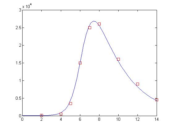
Not bad! Now, this may not actually be as good as our solution for our previous lesson. That’s ok. We’re only using 10 bits to represent each value and the GA is a randomized search process. One neat trick is that you can use the GA to find the correct basin of attraction and then use a gradient descent algorithm like nlinfit to get a more exact answer. I will not do that here.

Finally, I want to answer the question that was posed at the very beginning of Part 4A. I asked if we could figure out how long it takes people to recover from the infection based on our empirical data. Well, in fact, we can! In this case, our value for delta is the decay rate for people moving from the sick population to the recovered population. It just so happens that the inverse of the decay rate is the lifespan of the population. In this case: the lifespan of someone in the sick population. So, what is our answer?

>> 1/delta

ans =

    2.9693

Based on our model and our fit, we estimate that people recover from the illness in approximately 3 days! Good work! You made it. The next and last lesson in this five part series will be a little lighter on the math itself. We will take a look at complex systems and how sensitivity to initial conditions makes numerical prediction all but impossible! Until then, here are the files used in this lesson.

sir.m
ga.m
fitness.m
gene_to_values.m
squared_error.m

Thank you.