This is the final post in our series on random numbers in Matlab. In the first post, we discussed basic random number functions, and in the second post, we discussed the control of random number generation in Matlab and alternatives for applications with stronger requirements. In this post, we will demonstrate how to create probability distributions with the basic rand and randn functions of Matlab. This is useful in many engineering applications, including reliability analysis and communications.
How to Create More Distributions
Although the basic version of Matlab only provides the uniform and normal distributions, other distributions based on these functions can be generated. The log-normal, Rayleigh, and exponential distributions will be produced below as examples.
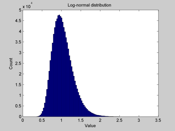
The log-normal distribution is easily.created by taking Euler’s number (e) to the power of a normal random variable (randn).
>> mu = 0;                %Mean of log(X)
>> sigma = 0.25;          %St. dev. of log(X)
>> N = 1000000;
>> nbins = 100;
>> X = exp(mu + sigma*randn(N,1));
>> hist(X, nbins);
>> xlabel('Value'); ylabel('Count');
>> title('Log-normal distribution')
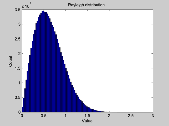
The Rayleigh distribution is commonly used to model wireless communication channels and can be constructed easily in Matlab. A Rayleigh random variable is the square root of the sum of the squares of two independent normal distributions with zero mean (randn).
>> sigma = 0.5;        %Scale parameter
>> N = 1000000;
>> nbins = 100;
>> X1 = sigma*randn(N,1);
>> X2 = sigma*randn(N,1);
>> R = sqrt(X1.^2 + X2.^2);
>> hist(R, nbins);
>> xlabel('Value'); ylabel('Count');
>> title('Rayleigh distribution')
The exponential distribution models the time between events in a Poisson process and can be created using the uniform distribution (rand).
>> lambda = 0.1;       %Rate parameter = 1/mean = 1/stdev
>> N = 1000000;
>> nbins = 100;
>> X = rand(N,1);
>> E = -log(X)/lambda;
>> hist(E, nbins);
>> xlabel('Value'); ylabel('Count');
>> title('Exponential distribution')

As shown in this post, creating distributions on the basis of the simple Matlab functions rand and randn is easy and requires only a few lines of code. This is highly useful for a wide range of engineering and scientific applications. I hope these posts have helped you learn about the Matlab random number functions and will enable you to apply them to your own work.
Very useful articles to many of my problems that I face when I did my homework.
Thank you
It is very useful to my homework… thank you
thank you
it was usefull
Run the attached script in MARLAB. this script generates N samples of z a gaussian distribution with mean mu and standard deviation sigma , denoted z~ N(mu,sigma2), and compares the sample histogram with Gaussian probability density function. familiaris yourself with the script by experimenting with different choices for N,mu, sigma and “dx”.
can any body tell how to do this
Using the below m file coding as a starting point, write a MATLAB code which generates N
samples from a Rayleigh distribution, and compares the sample histogram with the
Rayleigh density function. can anybody tell how to write from this starting?
% GAUSSIANHIST
clear
% Initialisation
mu = 0; % mean (mu)
sig = 2; % standard deviation (sigma)
N = 1e5; % number of samples
% Sample from Gaussian distribution
z = mu + sig*randn(1,N);
% Plot sample histogram, scaling vertical axis
% to ensure area under histogram is 1
dx = 0.5;
x = mu-5*sig:dx:mu+5*sig; % mean, and 5 standard
% deviations either side
H = hist(z,x);
area = sum(H*dx);
H = H/area;
bar(x,H)
xlim([-5*sig,5*sig])
% Overlay Gaussian density function
hold on
f = exp(-(x-mu).^2/(2*sig^2))/sqrt(2*pi*sig^2);
plot(x,f,’r’,’LineWidth’,3)
hold off
Very useful series of articles about random numbers in Matlab. Thank you.
Pingback: Random Numbers in Matlab – Part III | Business Intelligence Info