On Matlab Geeks, we have already covered basic two-dimensional plotting techniques. We would now like to start covering techniques for plotting three-dimensional data. One of the easiest and most visually pleasing ways of plotting three-dimensional data onto a 2-D surface is imagesc. Originally meant to be used with image data, this function is a great tool for plotting 2-D matrices. Imagesc is different from the image function in that the data is automatically scaled to fit the range of the colormap. This feature makes representing a matrix with imagesc is far easier than with image. We recommend using imagesc to plot data from a 2-D matrix.
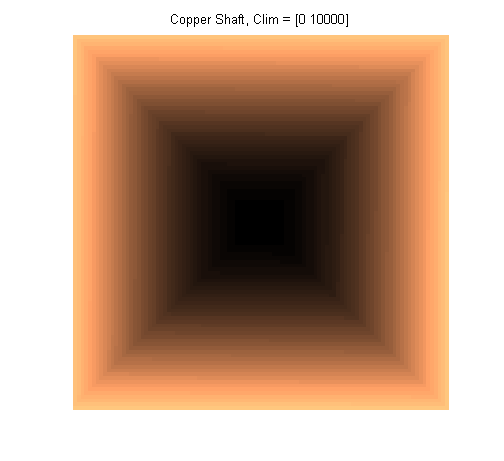
The following example shows how to plot a matrix using imagesc and how to change the color axis limits. This code creates what appears to be copper square shaft, which, visually, almost has a three-dimensional effect.
colormap copper
figure
imagesc(spiral(100))
axis square
axis off
title('Copper Shaft, Clim = [0 10000]')
The first figure shows the results of the above code. The function spiral creates a two-dimensional matrix that increases from 1 in the center to n^2 at the edge along a spiral path. Imagesc plots the matrix such that the data is spread evenly throughout the colormap.
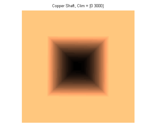
 The second figure was created by entering the following command:
set(gca,'Clim',[0 3000])
The center of the figure now shows more detail, but the figure is saturated at matrix values of 3000 or greater.
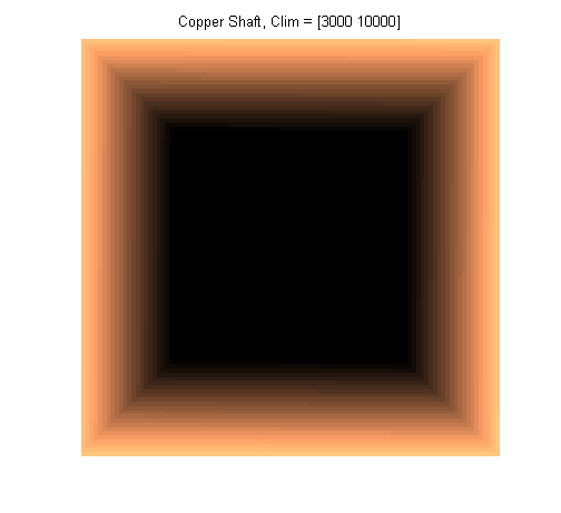
 The third figure shows the results of setting the color axis limits to [3000 to 10000]. The low values in the center of the figure are set to the lowest value of the colormap, while the edges of the figure show a greater amount of detail than in the original figure. The colormap has been set to correspond with values from 3000 to 10000, so there will be more colors for a smaller range of values, yielding more detail.
 Imagesc is a useful function that can be used to display 2-D data. The examples above turned off the axes, but normally the axes will be labeled starting from 1 and continuing to the number of data points in that dimension. To set the x- and y-coordinates, the following command can be used:
imagesc(10:10:1000,1:0.1:10,spiral(100))
This sets the x-coordinates to [10, 20, 30, … , 990, 1000], and the y-coordinates to [1, 1.1, 1.2, … , 9.9, 10]. This does not affect the size of the graph, but only changes the labels on the axes.
Imagesc is easy to use and allows a great deal of versatility when plotting data from a two-dimensional matrix. There is also no ambiguity about the values in the figure, which can be a problem with pcolor. No special preparation of the x- and y- coordinates is necessary either, unlike the mesh function. We recommend this function as a first choice for plotting a two-dimensional matrix.

Hi,
do you know if there is a way for Matlab to print the values found in the matrix in their corresponding square on the image?
Regards,
Nathan
Dear Sir/Madam
This blog is quite useful and now I am trying to plot curve data of X and Y coordinates on the image using plot and imagesc. However, i can see the plotted data on the image with different scaling.
Let say, my ROI(Region of Interest) is 188 x 210 pixels and the no of points in X and Y are 103 in each in terms of pixels. But the final figure shown in here http://imageshack.us/photo/my-images/822/finalcurvefittingforult.jpg/
is out of the original image edge. I think it will be because of scaling with plot and imagesc as well some reference starting points.
Pls advise me since I was stuck on it and looking forward to hearing from you good news soon.
Thanks and best regards
Kyaw