Check if a point is on a line segment

As we continue to look at different computational geometry problems, one simple, yet important test is to see whether a given point lies on a line segment. Similar to our previous posts, we will be utilizing the cross product and dot product to check for the proper conditions. Hopefully, these computations have become second nature now. Again, I have uploaded the script checkPointOnSegment.m if you want to test on your own.

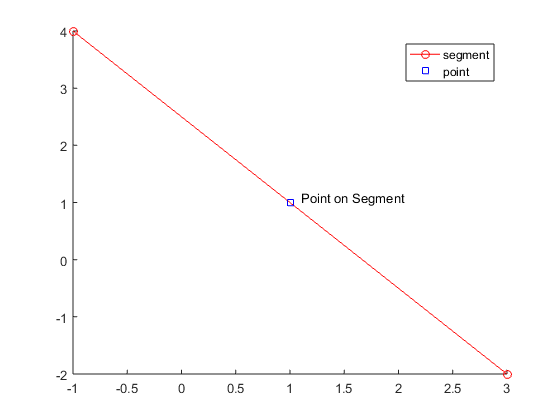
We will first define our segments and point of interest. Our segment will consist of a 2×2 array, with each row specifying each endpoint A and B, and a point C will be defined as a 2 element array. For example, given the following, we have a line from (-1,4) to (3,-2) and want to check if the point (1,1) lies on the segment.

>> segment = [-1 4; 3 -2];
>> C = [1 1];

Let’s now define the line segment as a vector from point A (-1,4) to point B(3,-2) and the vector AC:

A = segment(1,:);
B = segment(2,:);
% form vectors for the line segment (AB) and the point to one endpoint of
% segment
AB = B - A;
AC = C - A;

As we have shown previously, collinearity can be checked through the cross product. If the cross product of AB and AC is 0, then the segments have a 0 or 180 degree angle between them and are therefore collinear. We can do this simple check for whether a point is on a line, given our definition of cross. Note: if you use Matlab’s built-in cross, you’ll have to append 0’s to all of your vectors, but you will still obtain the same results.

% if not collinear then return false as point cannot be on segment
if cross(AB, AC) == 0
    checkPt = true;
end
%% Cross product returning z value
function z = cross(a, b)
    z = a(1)*b(2) - a(2)*b(1);

Alas, a line segment is different than a line, in that it has endpoints, while a line continues to infinity in both directions. So we need to perform some additional checks for whether the point is beyond the limits of the line segment. While we could do some simple > or < checks, let's use the dot product to see whether the point lies on the line segment or is found at the endpoints. So our complete code will be:

% if not collinear then return false as point cannot be on segment
if cross(AB, AC) == 0
    % calculate the dotproduct of (AB, AC) and (AB, AB) to see point is now
    % on the segment
    dotAB = dot(AB, AB);
    dotAC = dot(AB, AC);
    % on end points of segment
    if dotAC == 0 || dotAC == dotAB
        onEnd = true;
        checkPt = true;
    % on segment
    elseif dotAC > 0 && dotAC < dotAB
        checkPt = true;
    end
end

Let’s look at some examples. Please feel free to try on your own and let us know how it works for you.

[checkPt, onEnd] = checkPointOnSegment(segment, C, true)
checkPt =
  logical
   1

onEnd =
  logical
   0


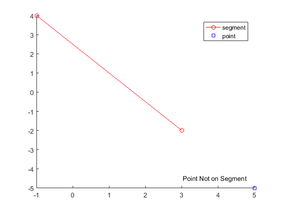
[checkPt, onEnd] = checkPointOnSegment(segment, [7,-5], true)
checkPt =
  logical
   0

onEnd =
  logical
   0

Equations for lines

In order to continue our discussion regarding polygons, points and other computational geometry code in MATLAB, we need to explain a few concepts.  This includes how we will describe points, vectors and lines.

A point is used to describe a location in Euclidean space, and in MATLAB we will use a one-dimensional array with n elements, with each element providing the location along each of the n dimensions. Such an array to describe a point in 3D space (at x = 1, y = 2, z = 3) might be as simple as:

p1 = [1,2,3]

Vectors, as opposed to points, provide both a magnitude and a direction. Unfortunately, in MATLAB the way to represent a vector is exactly the same as a point. Thus a vector a = <1,2,3> would also be written the same as p1 above, but would indicate that we have a vector point 1 unit in the x dimension, 2 units along y, and 3 units along z. In order to reduce confusion, ensure you properly comment your code and name your variables.

Finally, to describe a line, we will use two different methods. First, in 2-D space we can utilize the slope-intercept method. If given two points in Euclidean space, a line (segment) can be defined. Here is some sample code to generate the slope and intercept of the line. First lets initialize our function ‘getPointSlope’, and run checks to ensure proper definitions for the two points, ‘pointA’ and ‘pointB’.

function [slope, intercept] = getPointSlope(pointA, pointB, plotResults)
% Works in 2D space line defined by slope of the line (m) and the
% y-intercept (b), with the equation y = mx + b
if nargin < 3
    plotResults = false;
end
% error-check
if numel(pointA) ~=2 || numel(pointB) ~= 2
    error('The two points are not properly defined in 2-D space');
end

Next, there is a special condition, specifically vertical lines, where the slope-intercept method can break down. We need to check for this condition:

% Special condition when vertical line.  Will be the equation x = xA = xB:
if pointA(1) == pointB(1)
    slope = inf;
    intercept = pointA(1);
    warning(['Points provided define the line x = ', num2str(pointA(1))]);
    return
end

Note: In this condition, the output argument intercept is set to the x value, not the y-intercept. The user needs to ensure that if slope = inf, that the equation is x = intercept, rather than y = mx+b.

Next, we solve for the slope and intercept:

% Calculate the slope:
slope = (pointB(2) - pointA(2))/(pointB(1) - pointA(1));
% Solve for y-intercept
intercept = pointA(2) - slope*pointA(1);

Finally, if wanted, you can plot the results:

% plot the results
if plotResults
    figure; hold on;
    % plot the provided points
    plot([pointA(1) pointB(1)], [pointA(2) pointB(2)], 'bo');
    
    % calculate line y-values using mx+b equation we have solved for
    x0 = min([pointA(1) pointB(1)]) - 1;
    x1 = max([pointA(1) pointB(1)]) + 1;
    y0 = slope * x0 + intercept;
    y1 = slope * x1 + intercept;
    % plot the line
    plot([x0 x1], [y0 y1], 'r-');   
end

Here are a couple example results for two lines, the first one vertical (two points at [1,1] and [1,3]) and the second one through [1,1] and [2,3].  As you can see the results of the second line provide a slope (m) = 2 and a y-intercept (b) = -1:

While this slope-intercept form of a line is useful, and something you probably remember from grade school, another method we will use extensively is the paramaterized form.  In this form, each dimension is represented with the parametric equation x = x0 + at, y = y+bt, etc.  Here is some sample code that can quickly give you the values for a,b,c, etc based on the two points provided for the line:

function a = parameterizeLine(pointA, pointB)
% parameterized lines will have the form:
% x = x0 + a*t; 
% y = y0 + b*t;
% z = z0 + c*t; 
% etc
% where the output a to this function will be a vector of [a,b,c,...]
% [a,b,c] is the slope of the line.

% error check
if numel(pointA) ~= numel(pointB)
    error('points are not same dimensionality');
end
numDim = numel(pointA);
if numDim == 1
    error('1-D space');
end
% initialize a and solve
a = zeros(1, numDim);
for k = 1:numDim
    a(k) = pointB(k) - pointA(k);
end

We will be mostly using the parametric equation method for further posts, with t ranging from 0 to 1, but if you have any thoughts or comments, please let us know!