The basic premise of computational geometry is to calculate distances, areas, intersections and other geometrical calculations on basic objects such as points, lines and polygons. To begin this series on computational geometry in MATLAB, we’ll discuss the creation of random polygons in MATLAB.

In order to do so, we will compute points on the polygon by starting at the center of your choosing, traversing in a circle increasing the angle from 0 to 2pi (either clockwise or counter clockwise), assigning points on your polygon at a given radius away from the center, as represented by the following figure. The x and y points will then be calculated using x = r * cos(theta), y = r * sin(theta).

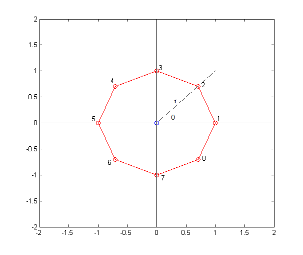
MATLAB Create Polygon

In this case, in order to create an equally spaced octagon, we have the center at (0,0), a radius of 1 unit and angle separations of pi/4. Here’s how we will set it up in MATLAB.

% Specify polygon variables
numVert = 8;
radius = 1;

% preallocate x and y 
x = zeros(numVert,1);
y = zeros(numVert,1);

% angle of the unit circle in radians
circleAng = 2*pi;
% the average angular separation between points in a unit circle
angleSeparation = circleAng/numVert;
% create the matrix of angles for equal separation of points
angleMatrix = 0: angleSeparation: circleAng;
% drop the final angle since 2Pi = 0
angleMatrix(end) = [];

Now we need to loop through all vertices that make up the polygon, initializing the x,y values to create the polygon.

% generate the points x and y
for k = 1:numVert
    x(k) = radius * cos(angleMatrix(k));
    y(k) = radius * sin(angleMatrix(k));
end

As you saw in the octagon created using this code, the polygon will always be convex and equally spaced, or a regular polygon. In order to generate non-regular polygons that may or not be concave or convex, you can add in some variability to the radius and angle separation measures. We will utilize the rand function to and this variability. Let’s start by initializing two new variables radVar and angVar to specify that we want variance in the radius and angle for each vertex.

% Specify polygon variables
numVert = 8;
radius = 1;
radVar = 1; % variance in the spikiness of vertices
angVar = 1; % variance in spacing of vertices around the unit circle

And now to calculate the x and y coordinates of each vertex on the polygon you can utilize new equations of x = (r+rVar) * cos(theta + thetaVar), y = (r + rVar) * sin(theta + thetaVar). In MATLAB code here is how these new x,y points will be calculated and plotted.

% generate the points x and y
for k = 1:numVert
    x(k) = (radius + radius*rand(1)*radVar) * cos(angleMatrix(k) + angleSeparation*rand(1)*angVar);
    y(k) = (radius + radius*rand(1)*radVar) * sin(angleMatrix(k) + angleSeparation*rand(1)*angVar);
end

% Graph the polygon and connect the final point to the first point
plot([x; x(1)],[y; y(1)],'ro-')
hold on
plot([-2 2],[0 0],'k')
plot([0 0],[-2 2],'k')

Here are some example 8 sided polygons that you might see.

As you can see in some instances the polygon will be convex and in others concave, but always 8-sided. If you want to play with the spikiness and spacing, play around with the “radVar” and “angVar” variables.