Random Walk in MATLAB for any Number of Dimensions

Previously, we showed how to perform a random walk in one dimension and in two dimensions using MATLAB’s rand function. Now let’s look at the general case, where the user can specify d > 1 dimensions and n >= 1 step. Here’s a sample gif of how this would look in three dimensions:


Continue reading

Two Dimensional Random Walk in MATLAB

Previously we described what a random walk is and demonstrated some simple code to perform this walk in one dimensional space. Today we will provide some simple code for how to perform such a walk in two-dimensional space. In the following post, we’ll look at the general case, and then we’ll get into some simulations. Here’s a sample of how our output will look like:

2D random walk in MATLAB

2D random walk in MATLAB

Continue reading

One dimensional random walk in MATLAB

We’re going to do a series of posts on Matlabgeeks to demonstrate how MATLAB is a wonderful option for running simulations. As a precursor to this, let’s look at a stochastic process known as a random walk. Briefly, such a process, in one-dimensional space, assumes equal probability of one of two possibilities occurring. For example, if you were to flip a fair coin multiple times, a random walk would demonstrate the total sum of heads and tails that are turned up after n flips. We will demonstrate how to model this process on the integer number line, with heads moving in the +1 direction and tails moving in the -1 direction.

Let’s first setup our function random_walk.m, taking in three input arguments:

% Random Walk in MATLAB
function position = random_walk(numSteps, numDimensions, plotResults)
% Vipul Lugade
% Oct 1, 2018
% matlabgeeks.com

% default values
if nargin < 3
    plotResults = false;
end
% Default the random walk to 2 Dimensions
if nargin < 2
    numDimensions = 2;
end
% Use 40 as default number of steps
if nargin < 1
    numSteps = 40;
end

The ‘numSteps’ variable specifies how many decisions (coin flips in 1D) to perform. The ‘numDimensions’ variable indicates how many dimensions to run the random walk across. For this post we will look at the simple case of 1 Dimensions, but we will show 2D/3D in a future post as well. Finally, the ‘plotResults’ variable is a boolean specifying whether to plot the results of the random walk.

In order to generate a random sequence of events, we will utilize MATLAB’s rand function, which we have previously discussed. For values < 0.5, we will set the value to -1 and for those greater than or equal to 0.5, we will set the value to 1.

% setup random walk values
randValues = round(rand(numSteps, numDimensions));

% One dimensional random walk
if numDimensions == 1
    randValues(randValues == 0) = -1;
% Two dimensional random walk
elseif numDimensions == 2
end

Now, perform the walk and calculate where on the number line we will be after n flips:

% start at origin and initialize the position
position = zeros(numSteps+1, numDimensions);
for k = 2:numSteps+1
    position(k,:) = position(k-1,:) + randValues(k-1,:);
end

Let’s look at an example, when running the following 1 dimensional random walk with 40 steps:

position = random_walk(40, 1, true)

One dimensional random walk in MATLAB

Stay tuned for further posts! If you have any comments or questions, don’t hesitate to contact us.

Check if a point is within a polygon – general case

Previously we had shown how to check if a two dimensional point is within a convex polygon. Now let’s look at the general case, where the polygon can be either convex or non-convex. To do so, we’ll use the ray casting algorithm. Briefly, this algorithm creates a ray or line segment from a point outside of the polygon to the point in question. Counting up the number of intersections, if the count is even (or zero), then the point lies outside of the polygon. Alternatively, if the count is odd, then the point is within the polygon.

So let’s create the general function pointWithinPolygon.m, which you can download and try yourself, to check if a given point is within a polygon defined by x and y coordinates px and py. This function will utilize the previously described checkSegmentIntersection and checkPointOnSegment functions. Once again we will define the polygon in either the clockwise or counterclockwise directions without repeating the first vertex. For the polygon, let’s define the following non-convex polygon as follows:

px = [0, 1,-1,-1,2,2,3,4];
py = [0, -1,-1,1,2,4,4,1];

First, let’s initialize our function and do some error checking to ensure proper definitions for the polygon and point of interest:

function insidePoly = pointWithinPolygon(px, py, point, plotResults)

if numel(px) ~= numel(py) || numel(px) < 3
    error('Incorrectly defined Polygon');
end
if numel(point) ~= 2
    error('Incorrectly defined point');
end

Now, to generate a count of how many segment intersections occur for a given ray from outside the polygon to the point in question, we first need to generate an outside point and the ray. To ensure that the outsidePoint is not within the polygon, we will utilize the minimum values minus one along all x and y of the polygon. The ray will be defined as an array from the defined outsidePoint to the point in question.

%% Generate ray from outside polygon to the point in question.
outsidePoint = [min(px) - 1, min(py) - 1];
ray = [outsidePoint; point];

The count for segment intersection will performed by looping through each edge of the polygon and checking if the given segment and ray will intersect. The intersection check will once again use the previously described checkSegmentIntersection code. A true value indicates that the ray intersects a segment and will lead to an increment in the count.

%% Check the intersection of each segment with the ray 
count = 0;
for k = 1:numel(px)
    if k < numel(px)
        doesIntersect = checkSegmentIntersection(ray, [px(k) py(k); px(k+1) py(k+1)], false);
    else
        doesIntersect = checkSegmentIntersection(ray, [px(k) py(k); px(1) py(1)], false);
    end
    if doesIntersect
        count = count + 1;
    end
end

This code is almost perfect… Unfortunately something goes horribly wrong when the ray passes through vertices of the polygon. For example, if we want to check the point (1,1) and select the outside point from (-2,-2), we will pass through the vertices (-1,-1) and (0,0), resulting in a count of 4, and incorrectly predicting that the point is outside the polygon:

To fix this problem, we’ll check if any vertices lie on the ray (using the code provided previously in checkPointOnSegment), and if they do, rotate the outside point until no vertices intersect the ray. This part of the code will have to be performed prior to the previously posted segment intersection check.

% ensure that ray does not intersect with polygon vertices and modify the
% outside point if it does so.
checkVert = true;
while checkVert
    for k = 1:numel(px)
        onRay = checkPointOnSegment(ray, [px(k), py(k)], false);
        if onRay
            outsidePoint = outsidePoint - rand(1,2);
            ray = [outsidePoint; point];
            break
        end
        if k == numel(px)
            checkVert = false; 
        end
    end
end

Now, our code should be robust with example results provided below. Please give the pointWithinPolygon.m code a try and let us know if you have any comments!

Check if a point is on a line segment

As we continue to look at different computational geometry problems, one simple, yet important test is to see whether a given point lies on a line segment. Similar to our previous posts, we will be utilizing the cross product and dot product to check for the proper conditions. Hopefully, these computations have become second nature now. Again, I have uploaded the script checkPointOnSegment.m if you want to test on your own.

We will first define our segments and point of interest. Our segment will consist of a 2×2 array, with each row specifying each endpoint A and B, and a point C will be defined as a 2 element array. For example, given the following, we have a line from (-1,4) to (3,-2) and want to check if the point (1,1) lies on the segment.

>> segment = [-1 4; 3 -2];
>> C = [1 1];

Let’s now define the line segment as a vector from point A (-1,4) to point B(3,-2) and the vector AC:

A = segment(1,:);
B = segment(2,:);
% form vectors for the line segment (AB) and the point to one endpoint of
% segment
AB = B - A;
AC = C - A;

As we have shown previously, collinearity can be checked through the cross product. If the cross product of AB and AC is 0, then the segments have a 0 or 180 degree angle between them and are therefore collinear. We can do this simple check for whether a point is on a line, given our definition of cross. Note: if you use Matlab’s built-in cross, you’ll have to append 0’s to all of your vectors, but you will still obtain the same results.

% if not collinear then return false as point cannot be on segment
if cross(AB, AC) == 0
    checkPt = true;
end
%% Cross product returning z value
function z = cross(a, b)
    z = a(1)*b(2) - a(2)*b(1);

Alas, a line segment is different than a line, in that it has endpoints, while a line continues to infinity in both directions. So we need to perform some additional checks for whether the point is beyond the limits of the line segment. While we could do some simple > or < checks, let's use the dot product to see whether the point lies on the line segment or is found at the endpoints. So our complete code will be:

% if not collinear then return false as point cannot be on segment
if cross(AB, AC) == 0
    % calculate the dotproduct of (AB, AC) and (AB, AB) to see point is now
    % on the segment
    dotAB = dot(AB, AB);
    dotAC = dot(AB, AC);
    % on end points of segment
    if dotAC == 0 || dotAC == dotAB
        onEnd = true;
        checkPt = true;
    % on segment
    elseif dotAC > 0 && dotAC < dotAB
        checkPt = true;
    end
end

Let’s look at some examples. Please feel free to try on your own and let us know how it works for you.

[checkPt, onEnd] = checkPointOnSegment(segment, C, true)
checkPt =
  logical
   1

onEnd =
  logical
   0


[checkPt, onEnd] = checkPointOnSegment(segment, [7,-5], true)
checkPt =
  logical
   0

onEnd =
  logical
   0

Find intersection of two lines in MATLAB

One computational geometry question that we will want to address is how to determine the intersection of two line segments. This will allow for further solutions for more complex questions, including a general solution regarding whether a point is inside or outside of a convex or non-convex polygon. Previously, we’ve described how to define a line segment in MATLAB, and we will use this definition in our current method for solving for line intersections.
Continue reading

Equations for lines

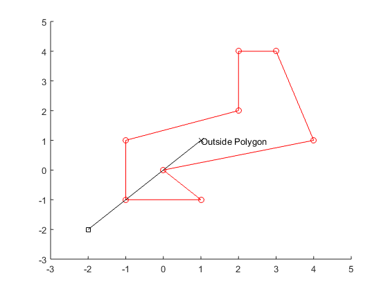
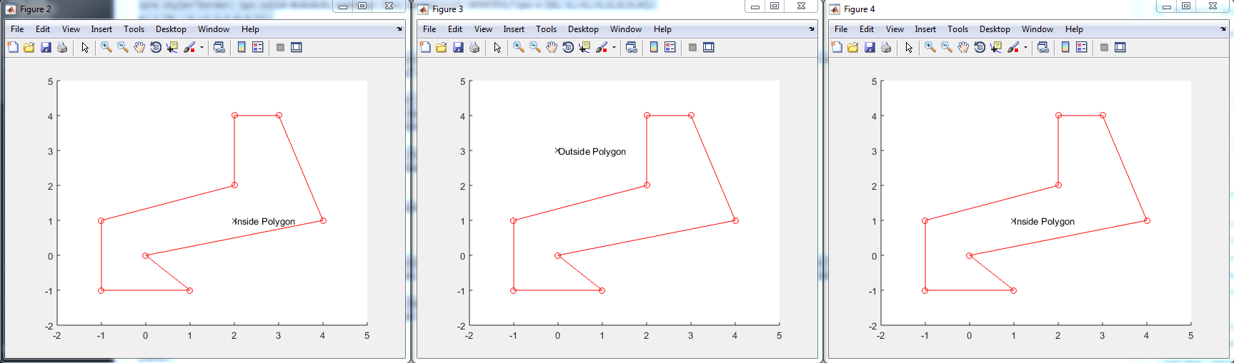
In order to continue our discussion regarding polygons, points and other computational geometry code in MATLAB, we need to explain a few concepts.  This includes how we will describe points, vectors and lines.

A point is used to describe a location in Euclidean space, and in MATLAB we will use a one-dimensional array with n elements, with each element providing the location along each of the n dimensions. Such an array to describe a point in 3D space (at x = 1, y = 2, z = 3) might be as simple as:

p1 = [1,2,3]

Vectors, as opposed to points, provide both a magnitude and a direction. Unfortunately, in MATLAB the way to represent a vector is exactly the same as a point. Thus a vector a = <1,2,3> would also be written the same as p1 above, but would indicate that we have a vector point 1 unit in the x dimension, 2 units along y, and 3 units along z. In order to reduce confusion, ensure you properly comment your code and name your variables.

Finally, to describe a line, we will use two different methods. First, in 2-D space we can utilize the slope-intercept method. If given two points in Euclidean space, a line (segment) can be defined. Here is some sample code to generate the slope and intercept of the line. First lets initialize our function ‘getPointSlope’, and run checks to ensure proper definitions for the two points, ‘pointA’ and ‘pointB’.

function [slope, intercept] = getPointSlope(pointA, pointB, plotResults)
% Works in 2D space line defined by slope of the line (m) and the
% y-intercept (b), with the equation y = mx + b
if nargin < 3
    plotResults = false;
end
% error-check
if numel(pointA) ~=2 || numel(pointB) ~= 2
    error('The two points are not properly defined in 2-D space');
end

Next, there is a special condition, specifically vertical lines, where the slope-intercept method can break down. We need to check for this condition:

% Special condition when vertical line.  Will be the equation x = xA = xB:
if pointA(1) == pointB(1)
    slope = inf;
    intercept = pointA(1);
    warning(['Points provided define the line x = ', num2str(pointA(1))]);
    return
end

Note: In this condition, the output argument intercept is set to the x value, not the y-intercept. The user needs to ensure that if slope = inf, that the equation is x = intercept, rather than y = mx+b.

Next, we solve for the slope and intercept:

% Calculate the slope:
slope = (pointB(2) - pointA(2))/(pointB(1) - pointA(1));
% Solve for y-intercept
intercept = pointA(2) - slope*pointA(1);

Finally, if wanted, you can plot the results:

% plot the results
if plotResults
    figure; hold on;
    % plot the provided points
    plot([pointA(1) pointB(1)], [pointA(2) pointB(2)], 'bo');
    
    % calculate line y-values using mx+b equation we have solved for
    x0 = min([pointA(1) pointB(1)]) - 1;
    x1 = max([pointA(1) pointB(1)]) + 1;
    y0 = slope * x0 + intercept;
    y1 = slope * x1 + intercept;
    % plot the line
    plot([x0 x1], [y0 y1], 'r-');   
end

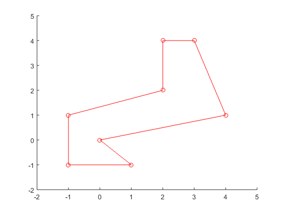
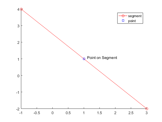
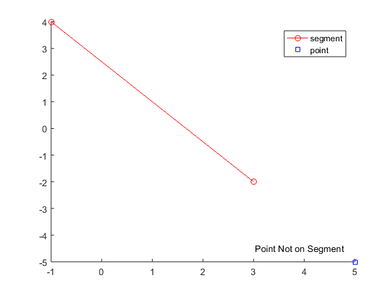
Here are a couple example results for two lines, the first one vertical (two points at [1,1] and [1,3]) and the second one through [1,1] and [2,3].  As you can see the results of the second line provide a slope (m) = 2 and a y-intercept (b) = -1:

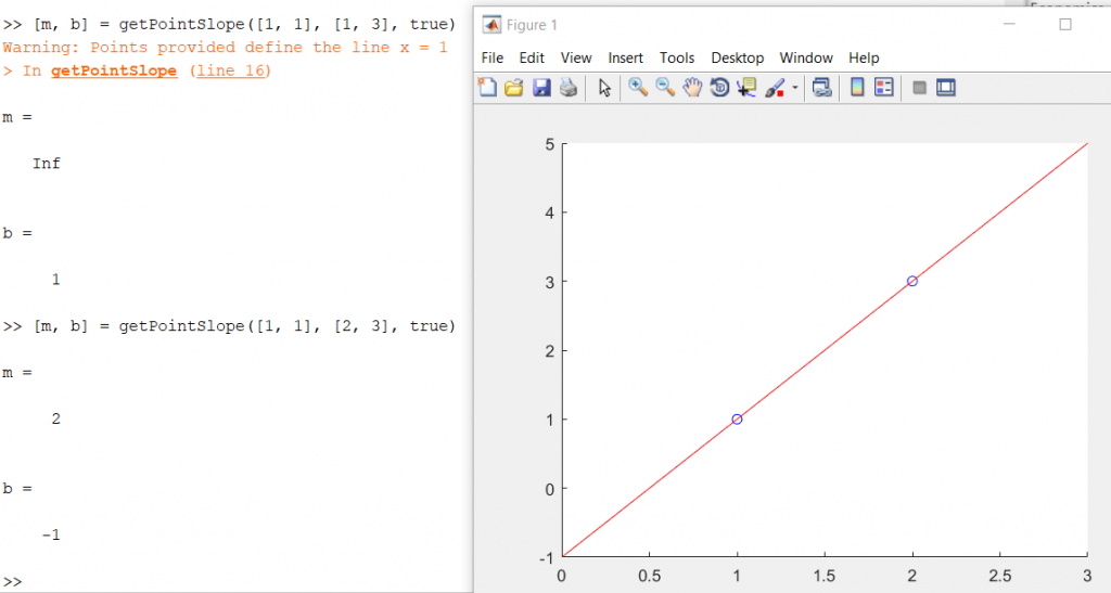
While this slope-intercept form of a line is useful, and something you probably remember from grade school, another method we will use extensively is the paramaterized form.  In this form, each dimension is represented with the parametric equation x = x0 + at, y = y+bt, etc.  Here is some sample code that can quickly give you the values for a,b,c, etc based on the two points provided for the line:

function a = parameterizeLine(pointA, pointB)
% parameterized lines will have the form:
% x = x0 + a*t; 
% y = y0 + b*t;
% z = z0 + c*t; 
% etc
% where the output a to this function will be a vector of [a,b,c,...]
% [a,b,c] is the slope of the line.

% error check
if numel(pointA) ~= numel(pointB)
    error('points are not same dimensionality');
end
numDim = numel(pointA);
if numDim == 1
    error('1-D space');
end
% initialize a and solve
a = zeros(1, numDim);
for k = 1:numDim
    a(k) = pointB(k) - pointA(k);
end

We will be mostly using the parametric equation method for further posts, with t ranging from 0 to 1, but if you have any thoughts or comments, please let us know!

Determine if a point is located within a convex polygon

It’s been a long time, but we are back again. We previously had discussed how to generate polygons by tracing a circle around a given center and placing vertices at randomly spaced angles and radii. Furthermore, we explained how to identify convexity of a given polygon. Continuing on this thread, we will explore how to determine whether a given point in space is inside or outside a given polygon. For this post, we will look at only convex polygons, but in a future post we will provide code to determine inside/outside for all cases.

Continue reading